


Introduction
Commonly known as the ‘King of Cereals’, wheat (Triticum aestivum L.) occupies the prime position among the food crops in the world. In India, it is the second most important food crop next to rice and contributes to the total food grain production of the country to the extent of about 25%. Currently, India is the second largest producer of wheat in the world after China, with around a 12% share in global wheat production. Indian wheat production in 2019-20 has made another landmark achievement by producing 107.18 million metric tons with an average national productivity of 3508 kg ha-1. The past year of production was also more than 100 million tons (103.60 million tons), and the current year of production has witnessed a change of 3.58 million tons (+3.46%). The positive production growth is attributed to the increased area of 4.21% despite a fall in the crop yield marginally by 0.72%. An increase in the support price also might have had a positive impact on the crop acreage (+1.24 million hectares). The average national productivity has crossed 3.5 t ha-1 for the first time in the country [1].
Production variability in cereal crops has been related to the availability of precipitation and temperatures during the growing season [2]. Crop productivity is primarily determined by a combination of temperature and precipitation because temperatures have to be in the optimum range for plant growth and precipitation has to supply crop water requirements for a given environment. The investigations have found decreased grain yield with exposure to high maximum temperatures, particularly at the later part of the crop growth. Temperatures impact crop phenology, and each species has a specific base temperature, an optimum temperature value, and an upper-temperature limit [3]. An increase in temperature above the optimum has shown a negative impact on wheat yield, with a projected 5.3% yield reduction per 1oC temperature rise [4]. High temperature following anthesis is called terminal heat, and continual stress is experienced by the crop when the mean daily temperature during pollination increases, and it has a significant impact on yield [5, 6]. Heat stress affects wheat production by reducing the tiller number, grain filling period, and grain size.
It is believed that wheat cultivation in India is a pure gamble of temperature. It has been presumed that increasing temperatures will become more significant in affecting wheat productivity in the coming years. However, some of this impact can be offset by ensuring these crops have an adequate soil water supply. Recent investigations [7, 8] suggest more attention to the effects of temperature on wheat productivity and suggest analyses and stimulation models be utilized for evaluating the potential growing regions and productivity for wheat under future climate scenarios.
Maintaining the appropriate sowing time is one of the most important agronomic practices for getting optimum plant growth and yield of wheat under heat-stressed environment [9], as in recent years we have experienced more fluctuations in temperature. Selection of suitable cultivars or genotypes can maintain higher productivity of wheat in any region. In general, late-sown wheat varieties face severe temperature stress, shortened heading, and maturity duration, and ultimately affect final yield and grain quality [10, 11]. Under the changing climate perspective, it is the need of the era to optimize the sowing window, which may have a great role in better performance of the crop. The low productivity of wheat in the eastern plains of India is due to a shorter favorable growing period, as in recent years, the temperatures began to rise from mid-February, and thus a short cool spell during its growing season with more fluctuation in temperature hampers the crop performance. Thus, the time of sowing is an important factor, and it is a non-cash input for achieving maximum yield. Advancing sowing time for a particular variety may not be always feasible in a high rainfall zone like the eastern sub-Himalayan plains of the country (India), where there is plenty of moisture in the soil even during the harvesting of the preceding rice crop in early November. Due to high residual moisture, the wheat crop can be grown successfully with a lower number of irrigations [12]. From an experiment conducted in the sub-Himalayan plains of India, it has been reported [13] that wheat sown on 25th November achieved maximum yield over the other dates of sowing; December 15 sowing recorded an estimated overall yield reduction of 40.7 kg ha-1 day-1 over November 25, sowing and at the same time, November 5 sowing also resulted in a yield decline by 42.7 kg ha-1 day-1, indicating the optimum sowing window in late November for eastern sub-Himalayan plains.
The deviation from the recommended sowing time of a variety for a particular set of environments results in failure to achieve its maximum production capacity. At the same time, we have to assess the suitability of varieties under various dates of sowing. The varieties performing better under timely sown conditions may not perform well under late or very late sown situations. Similarly, there are certain varieties that are well-responsive to restricted irrigation facilities. However, the variety having greater flexibility over the sowing dates would be of high priority, considering the practical situation of farming. Although the wheat varieties differ in maturity duration, still in the present study they have been considered together intentionally due to shifting of the climatic conditions of the zones in which the wheat varieties are recommended, under the present changing climatic conditions, since extremely low yields are predicted due to adverse weather conditions [14]. An increase in genetic diversity at the field level allows a greater resilience to climate variability [15]. A study of genetic variability for the characters showing responses to environmental conditions is a prerequisite for the adaptation of a population to an environment [16]. This adaptation is ensured by the presence or absence of genotype × environment (G×E) interaction, which largely determines the average response of the genotypes [17]. Temporal (over time in a single location) stability has been used along with spatial (over different locations) stability to understand the adaptation of the genotypes [16]. Some promising wheat varieties under timely sown irrigated, late, and very late sown, as well as rainfed conditions for this sub-Himalayan plain [18-20] have been identified previously. Both the macro and micro environmental factors have an important role to play in the study of the stability of wheat varieties in grain yield over varying environmental conditions. The macro environmental factors are uncontrollable and include the broad external conditions that affect plant breeding and agricultural practices like weather patterns, geography, soil type, and quality, pest and disease pressure, etc. On the other hand, the micro environmental factors are controllable and can be managed to some extent, like agricultural practices (sowing date), field management, microclimate (windbreaks, shelterbreaks, canopy management, etc.), soil microbiome (microbial diversity, organic matter), etc. The impact of macro and micro environments on a crop is best judged by studying the G×E interaction and selecting stable genotypes across different environmental conditions created due to changing climatic scenarios across the globe. Therefore, taking all these aspects into account and keeping in view the role of proper sowing time, which is a micro environmental and controllable factor in wheat production, the present experiment has been planned to study the genetic variability along with the G×E interaction of the wheat varieties and identify the potential varieties for this sub-Himalayan plain in India that have greater yield stability over varying sowing dates.
Materials and Methods
Experimental Site, Method, and Materials
The field experiment was conducted at the Instructional Farm of Uttar Banga Krishi Viswavidyalaya, Pundibari, Cooch Behar, located at 26o24’02.2” N latitude, 89o23’21.7” E longitude, and at an elevation of 43 meters above mean sea level (msl). It was carried out during the rabi (winter) seasons of two consecutive years, i.e., 2017-18 and 2018-19. The experimental site was bestowed with a sub-tropical humid climate. The soil of the experimental site was sandy loam in texture, acidic in reaction (pH 5.81), with an organic carbon content of 0.85%. The experimental soil was low in available nitrogen (238.9 kg ha-1), high in available phosphorus (32.6 kg ha-1), and medium in available potassium (146.8 kg ha-1). The meteorological monthly mean data pertaining to the period of experimentation are given in Table S1.
The experiment was laid out in a split-plot design with 24 treatment combinations, each replicated three times. Four different dates of sowing November 5th (D1), November 25th (D2), December 15th (D3), and January 5th (D4) were randomly allotted in each main plot, while six different wheat genotypes (HS 562, HD 2967, HD 3086, HI 1544, MACS 6222, WR 522) were randomly allocated in sub-plots. The important features of the varieties are mentioned in Table 1.
Agronomic Management
The seeds were sown manually in line with a seed rate of 100 kg ha-1 for D1 and D2, and 125 kg ha-1 for D3 and D4 at a row spacing of 20 cm. As the later sowing dates mostly result in decreased individual plant growth and tiller production, the seed rates under the later dates (D3 and D4) were 25% higher to maintain optimum stand count. The fertilizers were applied as per the recommendations of the All India Coordinated Wheat and Barley Improvement Project (AICW & BIP) under the Indian Council of Agricultural Research (ICAR), i.e., 150-60-40 kg ha-1 N-P2O5-K2O, respectively. The entire dose of P and K was applied as basal along with one-third of N. The rest N was applied in two equal splits, once at 21 days after sowing (DAS) and the next one at 42 DAS. Considering the deficiency of micronutrients (B and Zn in particular) in this tract, B was applied twice @ 0.20% with Soluble B (20% B), once at 35-40 DAS and the next at 55-60 DAS. Zinc (Zn) was applied at 0.10% with B in the second spray in the form of Chelated Zn. In both years, 4 irrigations were given at crown root initiation (CRI), active tillering, booting, and milking stages. Check basin method of irrigation was followed, keeping the depth of irrigation at 5 cm measured through volume basis. Harvesting of the crop was done manually and yield was estimated on a net plot basis excluding the border rows. After harvesting, the produce was threshed and grains were dried to record yield at 14% moisture.
Table 1.
Description of the wheat varieties taken in the experiment.
Data Collection
At harvest, the plant height was measured with a meter scale from the base to the tip of the plant. Five plants in each plot were randomly marked for this purpose except the border rows, and then the mean values were calculated and expressed in cm.
The days to maturity were counted from the date of seeding to the dates when the flag leaf and spike turned yellow. During the maturity stage, the number of spikes per square meter was randomly collected with the help of quadrates from five different spots in each plot, and accordingly, the mean values were calculated. The same procedure was followed for estimating the number of grains spike-1. Thousand-grain samples were collected separately from each plot after threshing and drying under the sun. After proper sun drying, the samples were put into a dryer (65-70ºC) for 2-3 days to take the final weights, and then the weight was expressed in grams for one thousand grains.
The entire produce from each net plot of twelve square meters was harvested (skipping the border rows) with the help of a sickle close to the ground level and then bundled separately and allowed to sun dry to reduce the moisture level. After proper sun drying, weight was taken, averaged, and converted into quintals per hectare. After the separation of grains, the straw obtained from each plot over the net plot used for grain yield estimation was properly dried under the sun, and then the weight of the entire biomass was recorded and expressed in terms of quintals ha-1 by considering both grain and straw.
Genetic Analysis for the Different Breeding Parameters and Statistical Analysis
The general statistical procedure was followed according to the standard method proposed [21]. The analysis of variance (ANOVA) and broad sense heritability (h2b) were estimated from the combined data over two years (2017-18 and 2018-19). The phenotypic coefficient of variation (PCV) and the genotypic coefficient of variation (GCV) were estimated according to the standard procedures [22]. The expected genetic advance (as a percentage of the mean) and the genotypic correlation were calculated [23]. The path analysis was carried out by the standard method [24]. The yield data was analyzed on an individual year basis and a combined basis, and the four different dates of sowing (D1, D2, D3, and D4) in the two years were treated to be a total of eight different environments (E1 to E8), considering the macro and micro environmental situations. So E1 was D1 in the first year of 2017-18, E2 was D2 in the first year of 2017-18, E3 was D3 in the first year of 2017-18, E4 was D4 in the first year of 2017-18, E5 was D1 in second year 2018-19, E6 was D2 in second year 2018-19, E7 was D3 in second year 2018-19, and E8 was D4 in second year 2018-19. The yield data was also used to estimate the different stability parameters as follows:
Regression-Based Stability Model
The stability model [25] deals with the regression approach to study the G × E interaction, and therein the interaction sum of squares is partitioned into two components. Among these two components, one component describes the heterogeneity of linear regression (bi), while the other component illustrates combined deviations from individual regression lines (S2di). The bi and the S2di are calculated as:
Where Xij is the performance of the ith genotype in the jth environment j, X̅i is the mean performance of the environment i, X̅j is the mean performance of the environment j, X̅i is the grand mean, and E is the number of environments. Depending upon the value of bi, the adaptability of the genotypes changes, i.e., when bi>1, the genotypes would be adapted to favorable environments, when bi<1, the genotypes would be adapted to unfavorable environmental conditions, and genotypes with bi = 1 would have an average adaptation to all environments. Genotypes with S2di = 0 would be most stable, whereas if S2di>0, it would indicate that the genotypes have lower stability across the environments. Overall, a genotype is said to be stable if the following conditions are fulfilled:
AMMI Stability Value (ASV)
In the AMMI model [26], the ASV is the difference between the coordinate point and the origin in a two-dimensional scatter diagram representing IPCA1 scores against IPCA2 scores. Because the IPCA1 score has more contribution to the G × E interaction sum of squares, a weighted value is needed. This weight is calculated for each genotype and each environment according to the relative contribution of IPCA1 to IPCA2 to the interaction sum of squares as follows:
Where
Yield Stability Index (YSI)
For the selection of a genotype, stability should not be the only parameter, as the most stable genotype might not necessarily give the best yield performance [27, 28]. Therefore, there is a requirement for integrating both mean yield and stability into a single selection index. So, the various authors and scientists proposed different selection criteria for the simultaneous selection of yield and stability [29-31]. In this context, the rank of ASV and the rank of the mean performance of a character are considered. The lowest ASV value occupies rank one, while the highest mean value of a character occupies rank one, and then both ranks are summed into a single selection index of stability, called the yield stability index (YSI) and that is considered the most stable as well as the highest yielding genotype.
Results
Variability Among the Wheat Genotypes over the Different Environments
The combined analysis of variance (Table 2) revealed that the six wheat genotypes differed significantly for grain yield and its attributing characters. The environments and the G×E interaction component also differed significantly for all the characters under study, indicating that the stability analysis of the wheat varieties can be further carried out in this study.
Genetic Variability
The study of genetic parameters (Table 3) showed wide variation in the range for all the characters. The grain yield ranged from 7.20 to 56.10 q ha-1 among the genotypes, which showed a large variation. The GCV (4.89 to 13.88) and PCV (4.89 to 14.61) values of the characters were low to moderate. The heritability values of the characters were quite high. The genetic advance values ranged from low to high.
Table 2.
Combined analysis of variance for the mean data of wheat genotypes over eight environments.
Table 3.
Genetic parameters (combined over eight environments) for the different yield-attributing characteristics of wheat.
Association between the Different Characters Indicating Their Influence on the Grain Yield
The genotypic correlation (Table S2) between grain yield and its attributing characters indicated that plant height was positively associated with days to physiological maturity (0.890**), spike per square meter (0.888**), grains per ear head (0.802*), biomass yield (0.765*), and grain yield (0.798*). The days to physiological maturity were positively associated with spike per square meter (0.872*), grains per ear head (0.943**), and grain yield (0.764*). Again, spike per square meter was positively associated with grains per spike (0.829*), biomass yield (0.994**), and grain yield (0.992**). Grains per spike were also positively associated with biomass yield (0.773*) and grain yield (0.840*). The character’s 1000-seed weight was not associated with any of the characters. Biomass yield was found to be positively associated with most of the characteristics like plant height (0.765*), spikes/m2 (0.992**), grains/ spike (0.840*), and grain yield (0.993**). In totality, grain yield was positively correlated with all the characters except 1000 seed weight.
Path Analysis for the Relationship between the Different Characters and Grain Yield
The path analysis (Table 4) measures the depth of the relationship between the different characters, which revealed that the highest direct effect on yield was exhibited by spike per square meter (1.216), which was closely followed by biomass yield (0.998) and grains per spike (0.633). These characteristics were also positively associated with grain yield, which indicated that any improvement in these three traits would result in a direct improvement in grain yield.
The correlation between plant height and grain yield (0.798) was significant and much higher than the direct effect of plant height (0.109) due to a negative indirect effect of plant height via days to physiological maturity. The correlation between days to physiological maturity and grain yield (0.764) was much higher than the direct effect of days to physiological maturity due to the indirect negative effect of days to physiological maturity via plant height. The correlation between spike per square meter and grain yield (0.992) was significant but lower than the direct effect of spike per square meter due to the negative indirect effect of spike per meter via plant height, days to physiological maturity, and 1000-seed weight. The correlation between grains per spike and grain yield (0.840) was higher than the direct effect of grains per spike (0.633), due to the greater negative indirect effect of grains per spike via days to physiological maturity (-1.547) and plant height (-0.088).
Table 4.
Direct (diagonal) and indirect (off-diagonal) effects (combined over eight environments) of different yield components on grain yield in wheat.
Table 5.
ANOVA for stability of the character grain yield of wheat over eight environments as per Eberhart and Russel (1966).
Ranking Based on Rescaled Index Value to Classify the Wheat Genotypes
The ranking of the genotypes (Table S3) based on the rescaled index value of the seven characters showed that the variety HD 2967 was the best performer with rank 1, followed by MACS 6222 (Rank 2), HI 1544 (Rank 3), HD 3086 (Rank 4), HS 562 (Rank 5), and WR 544 (Rank 6).
Stability Study Using Genotype ×
Environment Interaction
The ANOVA for stability (Table 5) as per Eberhart and Russel [25] for grain yield showed significance for genotypes and different components of the environment like [E+(G×E)], E, E (linear)] and the combined deviation, indicating a substantial difference between the varieties under study and the different environments created due to different dates of sowings and years.
The linear component of G×E differed significantly, which indicated that the performance of the wheat varieties could be predicted across the environments, created by the different dates of sowing and years, and the use of the stability parameters, i.e., bi (regression coefficient) and S2di (mean square deviation from linear regression), would be justified.
Eberhart and Russel (1966), AMMI and GGE Biplot Analysis
Based on mean grain yield over the environments (E1 to E8), regression coefficient (bi), and mean square deviation from linear regression (S2di) as per Eberhart and Russel [25] as mentioned in Table 6, it is clear that only HI 1544 showed non-significant bi and S2di, but its mean (27.221q ha-1) was lower than the population mean (27.831q ha-1). The other five varieties exhibited significant S2di along with non-significant bi, which did not give a clear indication regarding the stability of the varieties.
Table 6.
Mean grain yield of wheat genotypes in the individual eight environments (E1 to E8) and the stability parameters as per Eberhart and Russel (1966).
[i] Four different dates of sowing; November 5th (D1), November 25th (D2), December 15th (D3), and January 5th (D4). These four different dates of sowing (D1, D2, D3, and D4) in the two years were treated to be a total of eight different environments (E1 to E8), considering the macro and micro-environmental situations. So E1 was D1 in the first year of 2017-18, E2 was D2 in the first year of 2017-18, E3 was D3 in the first year of 2017-18, E4 was D4 in the first year of 2017-18, E5 was D1 in second year 2018-19, E6 was D2 in second year 2018-19, E7 was D3 in second year 2018- 19, and E8 was D4 in second year 2018-19. *Significant at 5% probability level, ** Significant at 1% probability level; Values in superscript in the format 1-6 indicate the respective ranks; Values in superscript in the format of a, b, ab, etc. indicate the DMRT values.
The heat map (Fig. 1) indicated the variable performance of the six wheat varieties over the eight environments created by the different dates of sowing over two years. The lighter shades in the heat map indicated higher yield and dark shades indicated lower yield. The stability analysis of the wheat varieties was further extended to AMMI and GGE Biplot analysis because the latter two techniques have additional advantages in providing more information and allowing greater discrimination among the varieties and their relationships between the environments [32]. The GGE biplot for discrimination and representativeness (Fig. 2) represents all the varieties in five environments, such as E3, E4, E5, E7, and E8, whereas the environments E1, E2, and E6 are highly differing and do not have much interaction with genotypes. The AMMI analysis of variance (Table S4) revealed that the replications, genotypes (varieties), environments, and G×E interactions component differed significantly for grain yield, which partially matched with the ANOVA of Eberhart and Russel model [25].
The AMMI analysis of variance (Table S4) for grain yield of the six wheat varieties showed highly significant differences among the genotypes and environments. The AMMI Stability Value (ASV) is calculated based on AMMI model IPCA1 and IPCA2 (interaction principal component 1 and 2, respectively) scores for each genotype. The varieties having the lowest ASV are considered widely adopted. The YSI (Yield Stability Index) is a more efficient indicator of stability as it combines high-yield performance along with stability. Lower YSI values indicate high yield along with greater stability (28, 30, and 31). Based on the ASV in the present study (Table 7), HI 1544 (Rank 1) was the most stable over the eight environments, followed by HS 562 (Rank 2) and HD 3086 (Rank 3). Based on YSI, it was found that HI 1544 (Rank 1) was the most stable and high-yielding variety, followed by HS 562 (Rank 2) and HD 2967 (Rank 3).
Ranking of Wheat Genotypes Based on Grain Yield Deviation in Different Environments
The study was further extended to the ranking of the wheat varieties based on the negative grain yield deviation from the mean in the eight environments (Table 8). An interesting observation here was that the most stable variety, HI 1544 (-38.618), was ranked fourth, and the other stable variety, MACS 6222 (-34.849), was ranked second in the list of total negative deviations of the six wheat varieties.
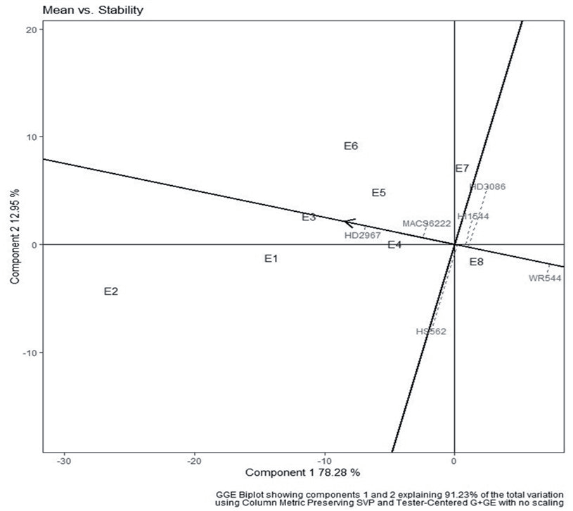
The GGE-biplot for the two principal components (Fig. 3) represented 91.23% of the variability. The environment and varieties were placed in all four quadrants (I, II, III, and IV). In quadrant I, the best performers were HD 2967 and MACS 6222, which were good in E3, E4, E5, and E6. In quadrant II, the best performers were HI 1544 and HD 3086 for E7. In quadrant III, the best performer was WR544 for E8 with less interaction. In quadrant IV, the highest yielder was HS562 for E1 and E2 with very little interaction. The environment closest to the origin was E4, followed by E8, E3, and E1, which implied that these environments were unfavorable for grain yield. The ranking of the wheat varieties by mean yield and stability is represented in Fig. 4. It revealed that the genotypes HD 2967 and MACS 6222 were placed closer to the origin, and it indicated a higher mean yield. The stability line (Y axis) indicated that HD1644, HD 3086, and HS 562 were the stable varieties. Since none of the varieties were placed away from the origin, it can be concluded that there was no greater G×E interaction and reduced stability.
Fig. 1.
Heat map for the performance of the different wheat genotypes for grain yield in the different environments. Note: Four different dates of sowing: November 5th (D1), November 25th (D2), December 15th (D3), and January 5th (D4). These four different dates of sowing (D1, D2, D3, and D4) in the two years were treated to be a total of eight different environments (E1 to E8), considering the macro and micro environmental situations. So E1 was D1 in the first year of 2017-18, E2 was D2 in the first year of 2017-18, E3 was D3 in the first year of 2017-18, E4 was D4 in the first year of 2017-18, E5 was D1 in the second year 2018-19, E6 was D2 in the second year 2018-19, E7 was D3 in the second year 2018-19, and E8 was D4 in the second year 2018-19.
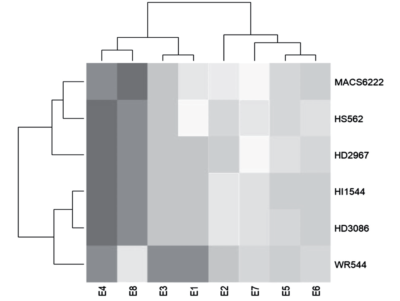
Fig. 2.
Discrimination versus representativeness. Note: Four different dates of sowing: November 5th (D1), November 25th (D2), December 15th (D3), and January 5th (D4). These four different dates of sowing (D1, D2, D3, and D4) in the two years were treated to be a total of eight different environments (E1 to E8), considering the macro and micro environmental situations. So E1 was D1 in the first year of 2017-18, E2 was D2 in the first year of 2017-18, E3 was D3 in the first year of 2017-18, E4 was D4 in the first year of 2017-18, E5 was D1 in the second year 2018-19, E6 was D2 in the second year 2018-19, E7 was D3 in the second year 2018-19, and E8 was D4 in the second year 2018-19.
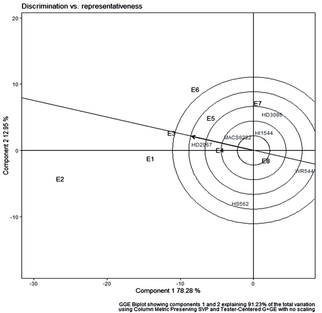
Table 7.
Ranking of six wheat genotypes based on grain yield, AMMI stability value (ASV), and yield stability index (YSI).
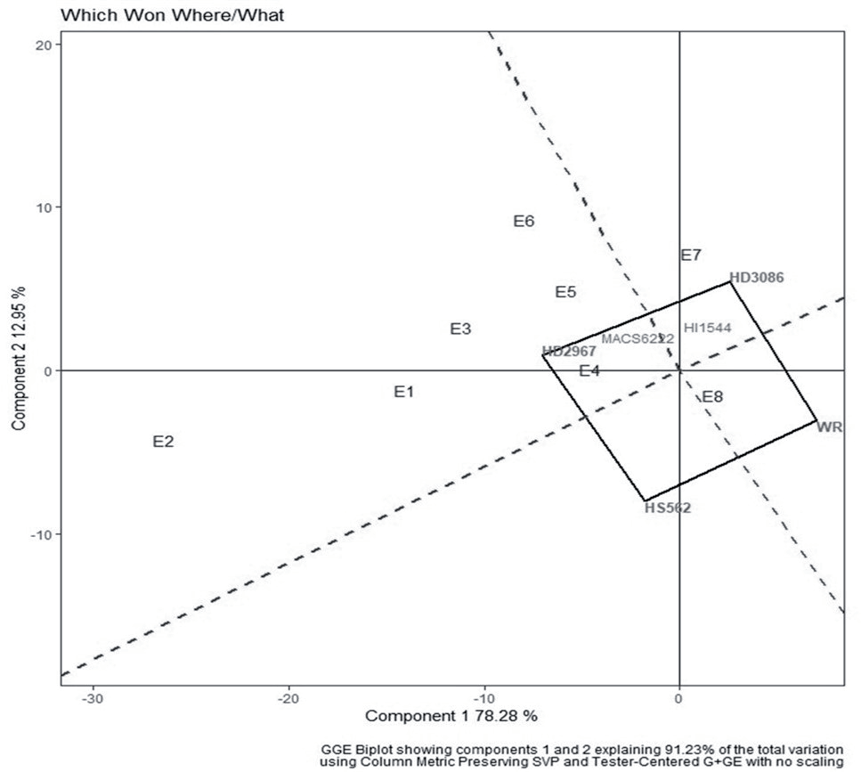
In the What-Won-Where biplot (Fig. 5), the four varieties HD 3086, WR 544, HS 562, and HD 2967 were placed at the vertices of a quadrilateral and the two environments (E4 and E8) in the three sectors. In sector III, the variety WR544 was the best performer for E8. HD 2967 from Sector I and HS 562 from Sector II were the best performers for E4. Sector II did not include any environment, and it can be concluded that varieties present in Sector II have no specific environment for recommendation.
Table 8.
Ranking of six wheat genotypes based on grain yield deviation from the mean in the eight environments.
[i] Values in superscript indicate the rank within the varieties for the negative deviations in yield. Four different dates of sowing: November 5th (D1), November 25th (D2), December 15th (D3), and January 5th (D4). These four different dates of sowing (D1, D2, D3, and D4) in the two years were treated to be a total of eight different environments (E1 to E8), considering the macro and micro environmental situations. So E1 was D1 in the first year of 2017-18, E2 was D2 in the first year of 2017-18, E3 was D3 in the first year of 2017-18, E4 was D4 in the first year of 2017-18, E5 was D1 in the second year 2018-19, E6 was D2 in the second year 2018- 19, E7 was D3 in the second year 2018-19, and E8 was D4 in the second year 2018-19.
Fig. 3.
GGE Biplot for PC1 and PC2. Note: Four different dates of sowing: November 5th (D1), November 25th (D2), December 15th (D3), and January 5th (D4). These four different dates of sowing (D1, D2, D3, and D4) in the two years were treated to be a total of eight different environments (E1 to E8), considering the macro and micro environmental situations. So E1 was D1 in the first year of 2017-18, E2 was D2 in the first year of 2017-18, E3 was D3 in the first year of 2017-18, E4 was D4 in the first year of 2017-18, E5 was D1 in the second year 2018-19, E6 was D2 in the second year 2018-19, E7 was D3 in the second year 2018-19, and E8 was D4 in the second year 2018-19.
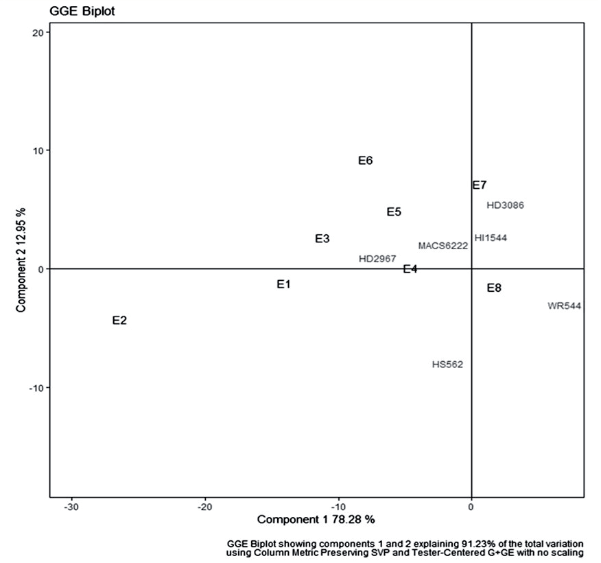
Fig. 4.
GGE for Mean versus Stability. Note: Four different dates of sowing: November 5th (D1), November 25th (D2), December 15th (D3), and January 5th (D4). These four different dates of sowing (D1, D2, D3, and D4) in the two years were treated to be a total of eight different environments (E1 to E8), considering the macro and micro environmental situations. So E1 was D1 in the first year of 2017-18, E2 was D2 in the first year of 2017-18, E3 was D3 in the first year of 2017-18, E4 was D4 in the first year of 2017-18, E5 was D1 in the second year 2018-19, E6 was D2 in the second year 2018-19, E7 was D3 in the second year 2018-19, and E8 was D4 in the second year 2018-19.
Discussion
Variability and Association Study between the Different Characters
A similar result regarding the variation in wheat genotypes was reported [33] in the evaluation of 11 wheat genotypes under eight locations in the North Hill zone of India. The same was also reported [34] in the evaluation of five potato clonal hybrids under six locations in Bangladesh. A similar report was shown [35] in a work on twenty wheat genotypes under nine test environments in Egypt, to determine the abiotic stress tolerance capacity. This indicated that there was sufficient variability in the genotypes and the environments and the interaction between them. The significance of the G×E interaction component indicated that the multi-environment performance of the genotypes can be further studied to assess their genetic potentiality for stability.
The GCV values were closer to the PCV values, indicating a lower effect of the environment on these characters. Similar views were opined [36] in a work on wheat genotypes for morpho-physiological characters. All the characters had high heritability, indicating the lower effect of the environment on these characters under study, and the GA was low to high for the different characters. The characters’ biomass yield and grain yield exhibited high heritability and genetic advance, which indicated that they are controlled by additive genes and would respond to selection.
In the linear regression analysis, a similar result of a positive correlation of biomass with grain yield was reported [37], while evaluating the effects of organic and inorganic fertilizers on wheat with five combinations of N, P, manure, and compost treatments, and it was concluded that grain yield was most strongly correlated with total biomass. This is also supported by another report [38], in a study in Iran extending for a period of several decades (from 1968 to 2018), involving 20 released spring wheat cultivars, which revealed that the wheat grain yield increased due to emphasis on traits like biomass, having a positive correlation with grain yield in combination with other agronomic traits. The association among the characters indicated that any improvement in most of the attributing characters except 1000-seed weight would result in an improvement of grain yield among the wheat genotypes under the present study.
Fig. 5.
Description of which won where what. Note: Four different dates of sowing: November 5th (D1), November 25th (D2), December 15th (D3), and January 5th (D4). These four different dates of sowing (D1, D2, D3, and D4) in the two years were treated to be a total of eight different environments (E1 to E8), considering the macro and micro environmental situations. So E1 was D1 in the first year of 2017-18, E2 was D2 in the first year of 2017-18, E3 was D3 in the first year of 2017-18, E4 was D4 in the first year of 2017-18, E5 was D1 in the second year 2018-19, E6 was D2 in the second year 2018-19, E7 was D3 in the second year 2018-19, and E8 was D4 in the second year 2018-19.
Due to the correlation between plant height and grain yield being significant and higher than the direct effect of plant height, therefore, direct selection for plant height will not improve the grain yield. In this case, direct selection for a higher spike per square meter would result in improved grain yield due to its higher direct effect. Also, direct selection for higher days to physiological maturity will not improve grain yield due to its very high negative direct effect on grain yield. In the case of biomass yield, its correlation with grain yield (0.993) was nearly similar to the direct effect of biomass yield, which was due to the internal cancellation of the positive and negative indirect effect of biomass yield via the other grain yield attributing characters. An interesting observation here was that plant height and days to physiological maturity created a negative indirect effect for the other grain yield attributing characters. On the other hand, spike per square meter and biomass yield created a positive indirect effect for the other grain yield attributing characters. The presence of a high residual effect in a population indicated the role of other possible independent variables that are not included in the study. In the present study, the residual effect of 0.2853 indicated that the characters presently studied fairly accounted for the total variability. The inclusion of a few more yield-attributing characters might have been better.
The inclusion of all the characters in the ranking (Table S3) of the varieties gave more clarity regarding their performance, not just based on grain yield, but also based on the grain yield attributing characters, and it helped to classify the wheat genotypes with HD 2967 with rank 1, followed by MACS 6222 (rank 2), and others. Interpretation of the results taking into consideration the ranking of the genotypes along with the stability parameters would throw more light on the adaptation of the genotypes across the environments created by different dates of sowing and years.
Stability of the Wheat Genotypes across the Environments
Genotype × environment (G×E) interaction is the result of the differences in sensitivities of the genotypes to the prevailing conditions in the target environment [39]. This is very pertinent under the present prevailing climate change conditions and the changes in the dates of sowing in a crop like wheat where the source-sink relationship keeps shifting, depending on the climatic conditions. As per Eberhart and Russel [25], a variety is said to be stable only if bi=1 and S2di=0 for that variety. Therefore, as per Table 6, strong conclusions could not be drawn regarding the stability of the varieties.
In the heat map (Fig. 1), the greater number of dark shades of HD 2967 in comparison to HI 1544 and MACS 6222 showed that HD 2967 suffered a greater degree of yield reduction with delay in sowing in the E4 and E8 (Table 8). However, HD 2967 was grouped along with the stable yielder MACS 6222 due to their higher average yields at rank 1 and 2, respectively, across the environments. Among the environments, it was found that those that were favorable (E2, E7, E5, and E6) with a positive environmental index were grouped into one, and those with a negative environmental index (E1, E3, E4, and E8) were grouped into another, thereby classifying the two distinct types of environments based on the sowing dates (Table 8). However, no specific trend in the yielding performance of the wheat varieties could be found, probably due to the variation in the responses of the varieties towards environmental fluctuations created by the changing dates of sowing over two years in combination with the changes in the weather parameter over the two years giving rise to complex interaction. Quite often the results of the Eberhart and Russel model [25] for stability do not match with those of AMMI and Biplot analysis due to the fact that AMMI and Biplot methods of stability analysis capture a much greater proportion of the genotype × environment (G×E) variance than the Eberhart and Russel method [40].
The AMMI model fits some of the several multiplicative forums instead of multiplicative forms in the assessment of varietal performance in varying environments [41]. The AMMI analysis (Table S4) determines the stability of the varieties across different environments using the PCA (Principal Component Analysis). Similar results of obtaining the lowest ASV with more stability were also reported [42] in fifteen rice genotypes under three different locations where the rice genotype SAHEL 108 (ASV = 0.05) was considered to be stable and possessed superior grain yield when compared to SAHEL 177 (ASV = 0.27). Similarly, in another evaluation of nineteen barley genotypes [43] under eight diverse locations, it was found that five barley genotypes KB 1405 (ASV = 0.33), BH 1013 (ASV = 0.57), BH 902 (ASV = 0.77), DWRB 150 (ASV = 1.14), and DWRB 101 (ASV = 1.32) with low ASV are stable across the environments when compared to RD 2941 (ASV = 3.63). An investigation [34] with five advanced potato genotypes evaluated under six locations in Bangladesh also showed that the potato genotype clone 9.125 (ASV = 0.50), followed by BARI Alu-28 (ASV = 0.56) and clones 9.91 (ASV = 0.67) were the most stable when compared to the clone 9.35 (ASV = 4.61), which is undesirable. In contrast to the result, it was found that the best-yielding genotype was the least stable, and the most stable genotype was placed in the lowest rank in spring wheat and cotton, respectively, which indicates that highly stable genotypes need not be high-yielding genotypes [44, 45].
A similar result of obtaining low YSI (Table 7) with high grain yield was also reported [46] in an experiment involving twenty-two advanced breeding lines of rice in twelve different salt-affected environments, where the rice genotypes STBN 22 (YSI = 0.989) and STBN 24 (YSI = 0.997) exhibited the highest mean grain yield with low yield stability index. Similarly, it has been reported [47] that the wheat genotypes with low YSI exhibit high grain yield while investigating 20 winter wheat genotypes under 24 environments in Iran. The Eberhart and Russell model [25] and the AMMI analysis revealed that the most stable varieties were HI 1544 and MACS 6222. The highest-yielding variety, HD 2967 (Rank 3) performed substantially better for stability as per the YSI ranking.
The two stable varieties, namely HI 1544 and MACS 6222, had exhibited low G×E interaction (Table 8) or a lower response to the environmental fluctuations arising out of different dates of sowing, starting from early (5th Nov.) to timely (25th Nov.) and then to late (15th Dec.) and very late (5th January) sowing, indicating a greater buffering capacity in them. On the other hand, the highest average yielding wheat variety, HD 2967 (34.05 q/ha), ranked 5th with a very high total negative deviation (-43.300), indicating a greater response to environmental fluctuations arising out of low buffering capacity.
The importance of the present study of well-known wheat varieties is enhanced by the fact that the best and the highest yielding variety HD 2967 in the first year exhibited the highest drop in grain yield from 51.700 q/ha in E2 (Nov. 25th sowing), which is a favorable environment, to 28.400 q ha-1in E3 (Dec. 15th sowing) and the lowest 15.867 q ha-1in E4 (Jan 5th sowing). Similarly, in the 2nd year, HD 2967 showed a steep drop from 47.933 q ha-1in E6 (25th Nov. sowing) to 18.800 q ha-1in E8 (5th Jan sowing), where E6 was the favorable environment of timely sown condition and E8 was the unfavorable late sown condition. Similar observations in the stable varieties HI 1544 and MACS 6222 did show a drop in the grain yield in E4 and E8 in the first and second years, but they were comparatively lower than the highest-yielding HD 2967. Another important observation was that in the most unfavorable environments E4 (Environmental index = -15.059) and E8 (Environmental index = -11.254), the negative deviation in yield was very high in the highest-yielding HD 2967 and quite low in the stable varieties HI 1544 and MACS 6222. This finding is in contrast to the finding from Table S3, where HD 2967 ranked first, followed by MACS 6222 (rank 2) and HI 1544 (rank 3), due to the masking effect of yield depreciation under unfavorable environments by the extremely high yield of HD 2967 under favorable environments. Hence, blind use of high-yielding wheat varieties over a large area with changing environmental and climatic conditions is not desirable. In wheat cultivation, any change in the sowing date or sowing window period for the sowing can have a devastating effect on grain yield as the yield reduction is to about 2/3rd with a realization of only 1/3rd of the potential yield in very high-yielding varieties with low buffering capacity, showing higher responsiveness to environmental fluctuations. This is extremely relevant to the present climate change scenario across the globe, where the climatic factors fluctuate every year as observed in the present study (Table S1) for temperature, relative humidity, total rainfall, and the number of rainy days.
The findings of some of the environments being unfavorable for grain yield (Fig. 3) are supported by the environmental index of the respective environments, E4 (-15.059), E8 (-11.254), E3 (-6.370), and E1 (-4320), which clearly states that the delayed sowing on January 5th of both years (E4 and E8), delayed sowing on Dec. 15th (E3), and early sowing (E1) in the first year caused a greater reduction in grain yield. According to Eberhart and Russel [25], a lower and negative environmental index for any environment means an unfavorable environment. On the other hand, the environments E6, E7, and E5 were away from the origin, indicating that they were favorable environments for grain yield. This is also supported by the higher environmental index in E6 (November 25th sowing in 2nd year), E7 (December 15th sowing in 2nd year), and E5 (November 5th sowing in 2nd year) with considerably high environmental mean deviation (Table 8).
Conclusions
The present two-year trial was successful in properly discriminating between the wheat varieties on the basis of their variable performance due to a change in the date of sowing, which is a micro environmental and controllable factor, by identifying the G×E interaction component under the different environments created. The use of different dates of sowing over two years and their treatment as different environments is fully justified by the wide range of environmental indexes of the different environments created, each of which also behaved differently in a favorable and unfavorable way with respect to grain yield. The present study revealed that the varieties HD 2967 and MACS 6222 were the superior performing ones for grain yield, out of which HD 2967 was a very high-yielding variety and performed well in E3, E4, and E5 environments but was also highly responsive to environmental fluctuations arising due to changes in dates of sowing. On the other hand, HI 1544 and MAC 6222 were identified as highly stable varieties performing well in almost all eight environments, with the least deviation in yield under unfavorable environments. Therefore, exploiting these varieties under the sub-Himalayan plains of India would ensure a high and stable grain yield.